
Since this post is a snapshot in time. I recommend that you download a copy of the book which is updated frequently to improve and expand the content.
---------------------------------------
This is the last of three posts working through a project looking at Measuring Recording and Exploring temperature measurements with the Raspberry Pi.
Explore
This section has a working solution for presenting multiple streams of temperature data. This is a slightly more complex use of JavaScript and d3.js specifically but it is a great platform that demonstrates several powerful techniques for manipulating and presenting data.
The final form of the graph should look something like the following (depending on the number of sensors you are using, and the amount of data you have collected)
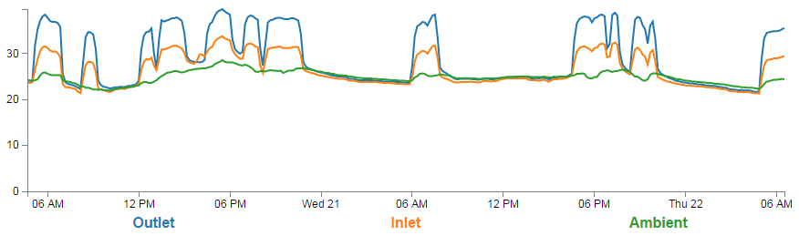
Multiple Line Graphs of Temperature
One of the neat things about this presentation is that it ‘builds itself’ in the sense that aside from us deciding what we want to label the specific temperature streams as, the code will organise all the colours and labels for us. Likewise, if the display is getting a bit messy we can click on the legend labels to show / hide the corresponding line.
The Code
The following code is a PHP file that we can place on our Raspberry Pi’s web server (in the /
var/www directory) that will allow us to view all of the results that have been recorded in the temperature directory on a graph; |
There are many sections of the code which have been explained already in the set-up section of the book that describes a simple line graph for a single temperature measurement. Where these occur we will be less thorough with the explanation of how the code works.
|
The full code can be found in the code samples bundled with this book (m_temp.php).
<?php

$hostname = 'localhost';
$username = 'pi_select';
$password = 'xxxxxxxxxx';

try {
    $dbh = new PDO("mysql:host=$hostname;dbname=measurements", $username, $pa\
ssword);

    /*** The SQL SELECT statement ***/

    $sth = $dbh->prepare("
       SELECT ROUND(AVG(`temperature`),1) AS temperature,
       TIMESTAMP(CONCAT(LEFT(`dtg`,15),'0')) AS date, sensor_id
       FROM `temperature`
       GROUP BY `sensor_id`,`date`
       ORDER BY `temperature`.`dtg` DESC
       LIMIT 0,900
    ");
    $sth->execute();

    /* Fetch all of the remaining rows in the result set */
    $result = $sth->fetchAll(PDO::FETCH_ASSOC);

    /*** close the database connection ***/
    $dbh = null;

}
catch(PDOException $e)
    {
        echo $e->getMessage();
    }

$json_data = json_encode($result);

?>
<!DOCTYPE html>
<meta charset="utf-8">
<style> /* set the CSS */
body { font: 12px Arial;}
path {
stroke: steelblue;
stroke-width: 2;
fill: none;
}
.axis path,
.axis line {
fill: none;
stroke: grey;
stroke-width: 1;
shape-rendering: crispEdges;
}
.legend {
font-size: 16px;
font-weight: bold;
text-anchor: middle;
}
</style>
<body>
<!-- load the d3.js library -->
<script src="http://d3js.org/d3.v3.min.js"></script>
<script>
// Set the dimensions of the canvas / graph
var margin = {top: 30, right: 20, bottom: 70, left: 50},
width = 900 - margin.left - margin.right,
height = 300 - margin.top - margin.bottom;
// Parse the date / time
var parseDate = d3.time.format("%Y-%m-%d %H:%M:%S").parse;
// Set the ranges
var x = d3.time.scale().range([0, width]);
var y = d3.scale.linear().range([height, 0]);
// Define the axes
var xAxis = d3.svg.axis().scale(x)
.orient("bottom");
var yAxis = d3.svg.axis().scale(y)
.orient("left").ticks(5);
// Define the line
var temperatureline = d3.svg.line()
.x(function(d) { return x(d.date); })
.y(function(d) { return y(d.temperature); });
// Adds the svg canvas
var svg = d3.select("body")
.append("svg")
.attr("width", width + margin.left + margin.right)
.attr("height", height + margin.top + margin.bottom)
.append("g")
.attr("transform",
"translate(" + margin.left + "," + margin.top + ")");
// Get the data
<?php echo "data=".$json_data.";" ?>
data.forEach(function(d) {
d.date = parseDate(d.date);
d.temperature = +d.temperature;
});
// Scale the range of the data
x.domain(d3.extent(data, function(d) { return d.date; }));
y.domain([0, d3.max(data, function(d) { return d.temperature; })]);
// Nest the entries by sensor_id
var dataNest = d3.nest()
.key(function(d) {return d.sensor_id;})
.entries(data);
var color = d3.scale.category10(); // set the colour scale
legendSpace = width/dataNest.length; // spacing for the legend
// Loop through each sensor_id / key
dataNest.forEach(function(d,i) {
svg.append("path")
.attr("class", "line")
.style("stroke", function() { // Add the colours dynamically
return d.color = color(d.key); })
.attr("id", 'tag'+d.key.replace(/\s+/g, '')) // assign ID
.attr("d", temperatureline(d.values));
// Add the Legend
svg.append("text")
.attr("x", (legendSpace/2)+i*legendSpace) // space legend
.attr("y", height + (margin.bottom/2)+ 5)
.attr("class", "legend") // style the legend
.style("fill", function() { // Add the colours dynamically
return d.color = color(d.key); })
.on("click", function(){
// Determine if current line is visible
var active = d.active ? false : true,
newOpacity = active ? 0 : 1;
// Hide or show the elements based on the ID
d3.select("#tag"+d.key.replace(/\s+/g, ''))
.transition().duration(100)
.style("opacity", newOpacity);
// Update whether or not the elements are active
d.active = active;
})
.text(
function() {
if (d.key == '28-00043b6ef8ff') {return "Inlet";}
if (d.key == '28-00043e9049ff') {return "Ambient";}
if (d.key == '28-00043e8defff') {return "Outlet";}
else {return d.key;}
});
});
// Add the X Axis
svg.append("g")
.attr("class", "x axis")
.attr("transform", "translate(0," + height + ")")
.call(xAxis);
// Add the Y Axis
svg.append("g")
.attr("class", "y axis")
.call(yAxis);
</script>
</body>
The graph that will look a little like this (except the data will be different of course).
Multiple Temperature Line Graph
This is a fairly basic graph (i.e, there is no title or labelling of axis). It will automatically try to collect 900 measurements. So if (as is the case here) we have three sensors, this will result in three lines, each of which has 300 data points.
It does include some cool things though.
- It will automatically include as many lines as we have data for. So if we have 7 sensors, there will be 7 lines.
- Currently the graph is showing the three lines in the legend as ‘Outlet’, ‘Inlet’ and ‘Ambient’. This is because our code specifically assigns a name to a sensor ID. But, if we do not assign a specific label it will automagically use the sensor ID as the label.
- The colours for the lines and the legend will automatically be set as nicely distinct colours.
- We can click on a legend label and it will turn on / off the corresponding line to make it easier to read.
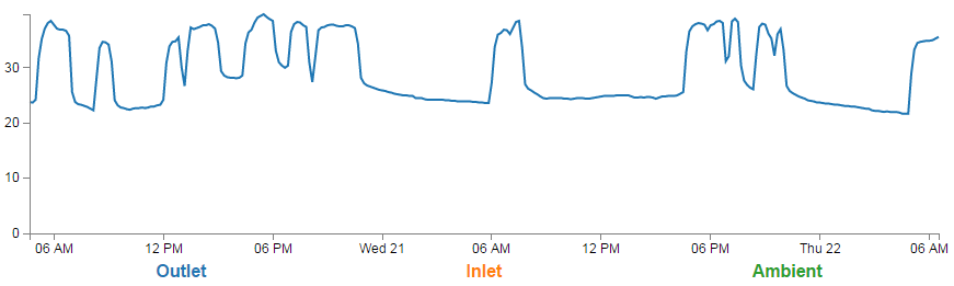
‘Inlet’ and ‘Ambient’ De-selected
PHP
The PHP block at the start of the code is mostly the same as our example code for our single temperature measurement project. The significant difference however is in the select statement.
       SELECT ROUND(AVG(`temperature`),1) AS temperature,
       TIMESTAMP(CONCAT(LEFT(`dtg`,15),'0')) AS date, sensor_id
       FROM `temperature`
       GROUP BY `sensor_id`,`date`
       ORDER BY `temperature`.`dtg` DESC
       LIMIT 0,900
The difference is that we are now selecting three columns of information. The temperature, the date-time-group and the sensor ID.
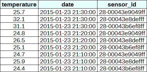
temperature date and sensor_id
In this project, we are going to need to ‘pivot’ the data that we are retrieving from our database so that it is produced in a multi-column format that the script can deal with easily. This is not always easy in programming, but it can be achieved using the d3
nestfunction which we will examine. Ultimately we want to be able to use the data in a format that looks a little like this;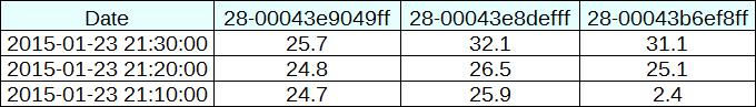
Pivoted sensor, temperature readings
We can see that the information is still the same, but there has been a degree of redundancy removed.
JavaScript
The code is very similar to our single temperature measurement code and comparing both will show us that we are doing the same thing in each graph, but the manipulation of the data into a ‘pivoted’ or ‘nested form is a major deviation.
Nesting the data
The following code nest’s the data
var dataNest = d3.nest()
 .key(function(d) {return d.sensor_id;})
 .entries(data);
We declare our new array’s name as
dataNest and we initiate the nest function;var dataNest = d3.nest()
We assign the
key for our new array as sensor_id. A ‘key’ is like a way of saying “This is the thing we will be grouping on”. In other words our resultant array will have a single entry for each unique sensor_id which will itself be an array of dates and values. .key(function(d) {return d.sensor_id;})
Then we tell the nest function which data array we will be using for our source of data.
}).entries(data);
Then we use the nested data to loop through our sensor IDs and draw the lines and the legend labels;
dataNest.forEach(function(d,i) {

 svg.append("path")
  .attr("class", "line")
  .style("stroke", function() { // Add the colours dynamically
   return d.color = color(d.key); })
  .attr("id", 'tag'+d.key.replace(/\s+/g, '')) // assign ID
  .attr("d", temperatureline(d.values));

 // Add the Legend
 svg.append("text")
  .attr("x", (legendSpace/2)+i*legendSpace)  // space legend
  .attr("y", height + (margin.bottom/2)+ 5)
  .attr("class", "legend")    // style the legend
  .style("fill", function() { // Add the colours dynamically
   return d.color = color(d.key); })
  .on("click", function(){
   // Determine if current line is visible
   var active   = d.active ? false : true,
   newOpacity = active ? 0 : 1;
   // Hide or show the elements based on the ID
   d3.select("#tag"+d.key.replace(/\s+/g, ''))
    .transition().duration(100)
    .style("opacity", newOpacity);
   // Update whether or not the elements are active
   d.active = active;
   })
  .text(
      function() {
          if (d.key == '28-00043b6ef8ff') {return "Inlet";}
          if (d.key == '28-00043e9049ff') {return "Ambient";}
          if (d.key == '28-00043e8defff') {return "Outlet";}
          else {return d.key;}
          });
});
The
forEach function being applied to dataNest means that it will take each of the keys that we have just declared with the d3.nest (each sensor ID) and use the values for each sensor ID to append a line using its values.
There is a small and subtle change that might other wise go unnoticed, but is nonetheless significant. We include an
i in the forEach function; dataNest.forEach(function(d,i) {
This might not seem like much of a big deal, but declaring
i allows us to access the index of the returned data. This means that each unique key (sensor ID) has a unique number.
Then the code can get on with the task of drawing our lines;
 svg.append("path")
  .attr("class", "line")
  .style("stroke", function() { // Add the colours dynamically
   return d.color = color(d.key); })
  .attr("id", 'tag'+d.key.replace(/\s+/g, '')) // assign ID
  .attr("d", temperatureline(d.values));
Applying the colours
Making sure that the colours that are applied to our lines (and ultimately our legend text) is unique from line to line is actually pretty easy.
The set-up for this is captured in an earlier code snippet.
var color = d3.scale.category10(); // set the colour scale
This declares an ordinal scale for our colours. This is a set of categorical colours (10 of them in this case) that can be invoked which are a nice mix of difference from each other and pleasant on the eye.
We then use the colour scale to assign a unique stroke (line colour) for each unique key (sensor ID) in our dataset.
    .style("stroke", function() {
        return d.color = color(d.key); })
It seems easy when it’s implemented, but in all reality, it is the product of some very clever thinking behind the scenes when designing d3.js and even picking the colours that are used.
Then we need to make sure that we can have a good reference between our lines and our legend labels. To do this we need to add assign an
id to each legend text label. .attr("id", 'tag'+d.key.replace(/\s+/g, ''))
Being able to use our
key value as the id means that each label will have a unique identifier. “What’s with adding the 'tag' piece of text to the id?” I hear you ask. Good question. If our key starts with a number we could strike trouble (in fact I’m sure there are plenty of other ways we could strike trouble too, but this was one I came across). As well as that we include a little regular expression goodness to strip any spaces out of the key with .replace(/\s+/g, ''). |
The
.replace calls the regular expression action on our key. \s is the regex for “whitespace”, and g is the “global” flag, meaning match ALL \s(whitespaces). The + allows for any contiguous string of space characters to being replaced with the empty string (''). This was a late addition to the example and kudos go to the participants in the Stack Overflow question here. |
Adding the legend
If we think about the process of adding a legend to our graph, what we’re trying to achieve is to take every unique data series we have (sensor ID) and add a relevant label showing which colour relates to which sensor. At the same time, we need to arrange the labels in such a way that they are presented in a manner that is not offensive to the eye. In the example I will go through I have chosen to arrange them neatly spaced along the bottom of the graph. so that the final result looks like the following;
Multi-line graph with legend
Bear in mind that the end result will align the legend completely automatically. If there are three sensors it will be equally spaced, if it is six sensors they will be equally spaced. The following is a reasonable mechanism to facilitate this, but if the labels for the data values are of radically different lengths, the final result will looks ‘odd’ likewise, if there are a LOT of data values, the legend will start to get crowded.
There are three broad categories of changes that we will want to make to our initial simple graph example code to make this possible;
- Declare a style for the legend font
- Change the area and margins for the graph to accommodate the additional text
- Add the text
Declaring the style for the legend text is as easy as making an appropriate entry in the
<style> section of the code. For this example we have the following;.legend {
font-size: 16px;
font-weight: bold;
text-anchor: middle;
}
To change the area and margins of the graph we can make the following small changes to the code.
var margin = {top: 30, right: 20, bottom: 70, left: 50},
    width = 900 - margin.left - margin.right,
    height = 300 - margin.top - margin.bottom;
The bottom margin is now 70 pixels high and the overall space for the area that the graph (including the margins) covers is increased to 300 pixels.
To add the legend text is slightly more work, but only slightly more.
One of the ‘structural’ changes we needed to put in was a piece of code that understood the physical layout of what we are trying to achieve;
legendSpace = width/dataNest.length; // spacing for the legend
This finds the spacing between each legend label by dividing the width of the graph area by the number of sensor IDs (
key’s).
The following code can then go ahead and add the legend;
 // Add the Legend
 svg.append("text")
  .attr("x", (legendSpace/2)+i*legendSpace)  // space legend
  .attr("y", height + (margin.bottom/2)+ 5)
  .attr("class", "legend")    // style the legend
  .style("fill", function() { // Add the colours dynamically
   return d.color = color(d.key); })
  .on("click", function(){
   // Determine if current line is visible
   var active   = d.active ? false : true,
   newOpacity = active ? 0 : 1;
   // Hide or show the elements based on the ID
   d3.select("#tag"+d.key.replace(/\s+/g, ''))
    .transition().duration(100)
    .style("opacity", newOpacity);
   // Update whether or not the elements are active
   d.active = active;
   })
  .text(
      function() {
          if (d.key == '28-00043b6ef8ff') {return "Inlet";}
          if (d.key == '28-00043e9049ff') {return "Ambient";}
          if (d.key == '28-00043e8defff') {return "Outlet";}
          else {return d.key;}
          });
There are some slightly complicated things going on in here, so we’ll make sure that they get explained.
Firstly we get all our positioning attributes so that our legend will go into the right place;
  .attr("x", (legendSpace/2)+i*legendSpace)  // space legend
  .attr("y", height + (margin.bottom/2)+ 5)
  .attr("class", "legend")    // style the legend
The horizontal spacing for the labels is achieved by setting each label to the position set by the index associated with the label and the space available on the graph. To make it work out nicely we add half a
legendSpace at the start (legendSpace/2) and then add the product of the index (i) and legendSpace (i*legendSpace).
We position the legend vertically so that it is in the middle of the bottom margin (
height + (margin.bottom/2)+ 5).
And we apply the same colour function to the text as we did to the lines earlier;
  .style("fill", function() { // Add the colours dynamically
   return d.color = color(d.key); })
Making it interactive
The last significant step we’ll take in this example is to provide ourselves with a bit of control over how the graph looks. Even with the multiple colours, the graph could still be said to be ‘busy’. To clean it up or at least to provide the ability to more clearly display the data that a user wants to see we will add code that will allow us to click on a legend label and this will toggle the corresponding graph line on or off.
  .on("click", function(){
   // Determine if current line is visible
   var active   = d.active ? false : true,
   newOpacity = active ? 0 : 1;
   // Hide or show the elements based on the ID
   d3.select("#tag"+d.key.replace(/\s+/g, ''))
    .transition().duration(100)
    .style("opacity", newOpacity);
   // Update whether or not the elements are active
   d.active = active;
   })
We use the
.on("click", function(){ call to carry out some actions on the label if it is clicked on. We toggle the .active descriptor for our element with var active = d.active ? false : true,. Then we set the value of newOpacity to either 0 or 1 depending on whether active is false or true.
From here we can select our label using its unique id and adjust it’s opacity to either
0(transparent) or 1 (opaque); d3.select("#tag"+d.key.replace(/\s+/g, ''))
.transition().duration(100)
.style("opacity", newOpacity);
Just because we can, we also add in a
transition statement so that the change in transparency doesn’t occur in a flash (100 milli seconds in fact (.duration(100))).
Lastly we update our
d.active variable to whatever the active state is so that it can toggle correctly the next time it is clicked on.
Since it’s kind of difficult to represent interactivity in a book, head on over to the live example on bl.ocks.org to see the toggling awesomeness that could be yours!
Printing out custom labels
The only thing left to do is to decide what to print for our labels. If we wanted to simply show each sensor ID we could have the following;
.text(d.key);
This would produce the following at the bottom of the graph;

Multi-line graph with legend
But it makes more sense to put a real-world label in place so the user has a good idea about what they’re looking at. To do this we can use an
if statement to match up our sensors with a nice human readable representation of what is going on; .text(
function() {
if (d.key == '28-00043b6ef8ff') {return "Inlet";}
if (d.key == '28-00043e9049ff') {return "Ambient";}
if (d.key == '28-00043e8defff') {return "Outlet";}
else {return d.key;}
});
The final result is a neat and tidy legend at the bottom of the graph;
Multi-line graph with legend
The post above (and heaps of other stuff) is in the book 'Raspberry Pi: Measure, Record, Explore' that can be downloaded for free (or donate if you really want to :-)).
No comments:
Post a Comment